This notebook examines how case volumes changed across the three operational periods, with the goal of establishing the impact of self-serve automation on the volume. The focus is on what the automation deflected and what were the downstream effects created for the remaining caseload.
There is a summary section at the end of this.
Setup - Similar Setup in Each Notebook
The setup is to load the data in each notebook so that they can run individually as well.
Code
# Import necessary librariesimport osimport numpy as npimport pandas as pdimport matplotlib.pyplot as pltimport seaborn as snsfrom scipy.stats import chi2_contingency, gaussian_kdefrom statsmodels.stats.proportion import proportions_ztestimport warningswarnings.filterwarnings("ignore")# Set plt styleplt.style.use("ggplot")# Load the operations cases and reviews dataops_cases_df = pd.read_csv("ops_cases.csv")ops_reviews_df = pd.read_csv("ops_reviews.csv")
Code
# Define correct period order for the analysisperiod_order = ["Baseline", "Self-serve Only", "Both Changes"]ops_cases_df["period"] = pd.Categorical( ops_cases_df["period"], categories=period_order, ordered=True)
1. Overall Volume Trend
Daily and weekly Volume Trends
Daily Volume Trends
Code
# Create a date column and group the data by date to create a daily case count dataops_cases_df["date"] = pd.to_datetime(ops_cases_df["created_at"]).dt.datedaily_case_count_df = ops_cases_df[["case_id", "date"]].groupby("date").count()# Describe the dataframe to understand some basic statistical valuesdaily_case_count_df.describe().round(2)
case_id
count
180.00
mean
71.34
std
12.93
min
38.00
25%
61.00
50%
70.00
75%
82.25
max
103.00
Code
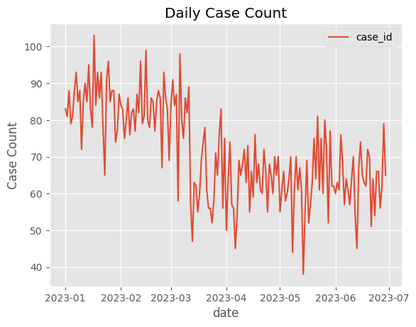
# Plot the volume trend of the datadaily_case_count_df.plot(ylabel="Case Count", title="Daily Case Count")
Weekly Volume Trends
Code
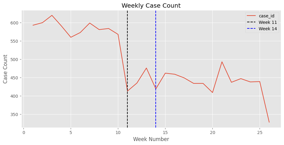
# Plot the weekly trend of the data using the week number columnweekly_case_count_df = ( ops_cases_df[["case_id", "week_number"]].groupby("week_number").count())# Plot the weekly graph and specifically mark Week 11 and Week 14weekly_case_count_df.plot( xlabel="Week Number", ylabel="Case Count", title="Weekly Case Count", figsize=(11, 5),)plt.axvline(x=11, color="black", linestyle="--", label="Week 11")plt.axvline(x=14, color="blue", linestyle="--", label="Week 14")plt.legend()plt.show()
2. Volume by Queue Type
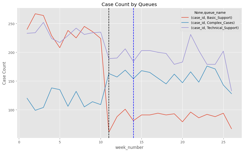
Segmenting by queue reveals which case types were affected by self-serve automation.
Code
# Review if there were any volume trends by categorical variables like queue_name and initial_handler_type as well as the periodqueue_name_volume_df = ( ops_cases_df[["case_id", "queue_name", "week_number"]] .groupby(["queue_name", "week_number"], as_index=False) .count())queue_name_volume_df.pivot(index="week_number", columns="queue_name").plot( figsize=(12, 7), ylabel="Case Count", title="Case Count by Queues")plt.axvline(x=11, color="black", linestyle="--", label="Week 11")plt.axvline(x=14, color="blue", linestyle="--", label="Week 14")
Code
# Review the pre and post self-serve changeweekly_counts = queue_by_week_df.reset_index()weekly_counts["period_self_serve"] = weekly_counts["week_number"].apply(lambda x: "pre"if x <11else"post")# Define correct period order for the analysisweekly_counts["period_self_serve"] = pd.Categorical( weekly_counts["period_self_serve"], categories=["pre", "post"], ordered=True)# Average cases by period and queue to create a tableweekly_counts.groupby("period_self_serve", as_index="False")[ ["Basic_Support", "Complex_Cases", "Technical_Support"]].mean().round(1)
queue_name
Basic_Support
Complex_Cases
Technical_Support
period_self_serve
pre
237.6
116.2
233.1
post
87.1
157.3
191.4
3. Queue Mix Shift Pattern
Code
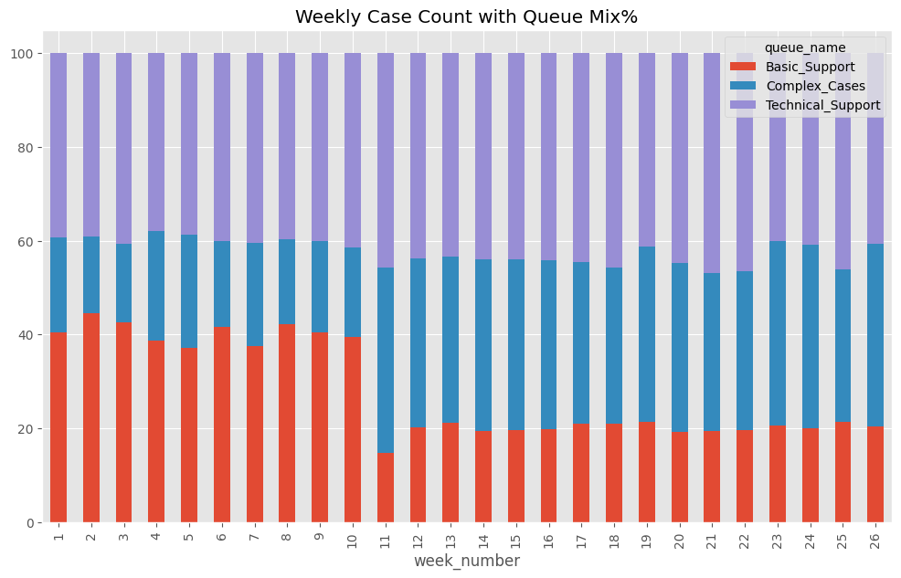
# Pivot to the weekly format with columns as queue namequeue_by_week_df = queue_name_volume_df.pivot( index="week_number", columns="queue_name", values="case_id")# Create a df with a percentage queue mix adding up to 100%queue_mix_pct_df = queue_by_week_df.div(queue_by_week_df.sum(axis=1), axis=0) *100# Explore the queue mix week on week to review what was the composition of the cases each weekqueue_mix_pct_df.plot( kind="bar", stacked=True, title="Weekly Case Count with Queue Mix%", figsize=(12, 7))plt.show()
4. Volume by Handler Type
Code
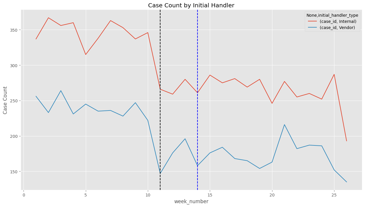
# Review if there were any volume trends by categorical variables like queue_name and initial_handler_type as well as the periodinit_handler_type_volume_df = ( ops_cases_df[["case_id", "initial_handler_type", "week_number"]] .groupby(["initial_handler_type", "week_number"], as_index=False) .count())init_handler_type_volume_df.pivot( index="week_number", columns="initial_handler_type").plot(figsize=(15, 8), ylabel="Case Count", title="Case Count by Initial Handler")plt.axvline(x=11, color="black", linestyle="--", label="Week 11")plt.axvline(x=14, color="blue", linestyle="--", label="Week 14")
Volume Analysis Summary
The total case volume dropped ~27% following the self-serve automation launch at Week 11. It went from ~580 cases/week in the baseline period to ~420 cases/week post-launch, where it broadly stabilised. The Week 14 routing change doesn’t seem to have much impact on the volume as such. This is expected because routing only changed how cases were assigned, not how many arrived in the queue.
While the decline might seem like a great thing at the surface, it seems to be primarily driven by Basic_Support Queue Type. Cases in this queue fell from ~240/week to ~90/week after Week 11, while the Technical_Support volumes held roughly steady. On the other hand, Complex_Cases overall increased in volume. The takeaway is that Self-serve automation started deflecting only simpler cases out of the agent queue but still maintained the technical and complex cases in their queue.
This creates a potentially unintended outcome - a structural complexity mix shift. Basic_Support’s share of total volume halved from ~40% to ~20%, while Complex_Cases grew from ~20% to ~35%. The caseload agents were seeing was harder on average and harder cases take longer to resolve.
Finally, the volume drop was proportional across handler types — both internal and vendor case counts fell by similar magnitudes at Week 11. This means vendor teams weren’t selectively affected by self-serve, making them a relatively clean control group for the routing change analysis later.
Next: Review SLA performance over time. We will break them down by handler type and queue. Given the mix shift we’ve just seen, we need to understand how much of the SLA decline is explained by agents now inheriting a harder caseload, versus something the routing change specifically introduced for internal teams.