This section examines how the Average Handle Time (AHT) and Average Speed of Answer (ASA) were impacted over the weeks due to different operational changes. It should hopefully confirm some analysis about the previous sections. We introduce some key metrics here.
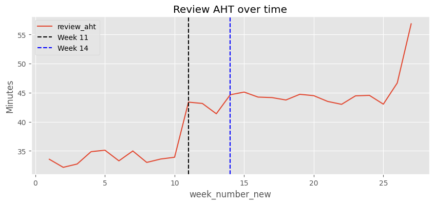
Review AHT - Mean time (in minutes) an agent actively works on a review. This is calculated as end_at - intended_start_at
Case AHT - Mean time (in hours) it takes to complete a case from start to finish (including all reviews)
Average Speed of Answer (ASA) - It’s the time taken from a case reaching the queue to when it’s finally worked on. This will be calculated from the review table as the difference between actual_start_at - intended_start_at. There can be two potential metrics here:
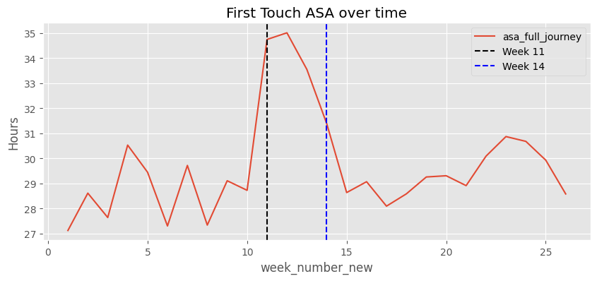
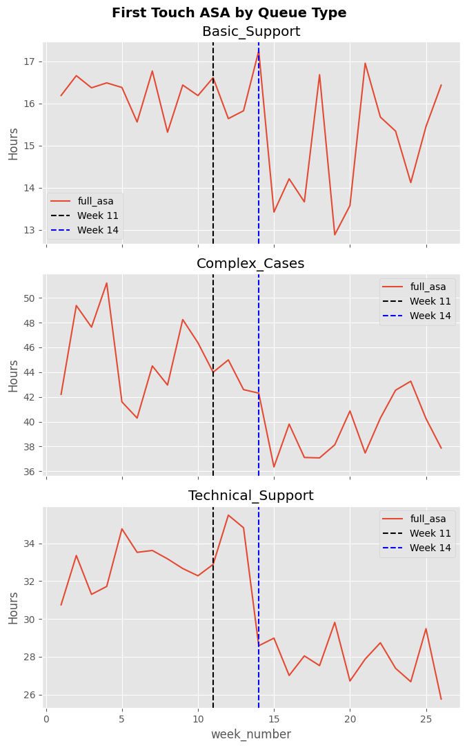
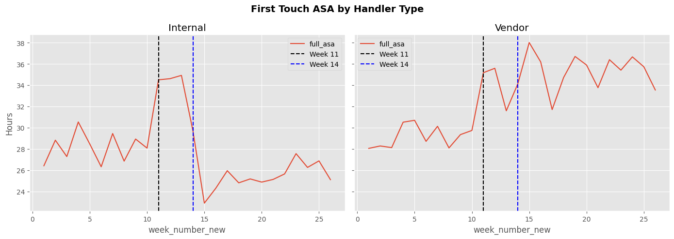
First Touch ASA = Average of actual_start_at - intended_start_at for all cases where review_order = 1
Full Journey ASA = Average of actual_start_at - intended_start_at for all cases
There is a detailed summary section at the end.
Imports and Setup
This is similar across all files
Code
# Import librariesimport numpy as npimport pandas as pdimport matplotlib.pyplot as pltfrom scipy.stats import gaussian_kdeimport warningswarnings.filterwarnings("ignore")# Set plt styleplt.style.use("ggplot")# Load the operations cases and reviews dataops_cases_df = pd.read_csv("ops_cases.csv")ops_reviews_df = pd.read_csv("ops_reviews.csv")# Set the period order for the dataperiod_order = ["Baseline", "Self-serve Only", "Both Changes"]ops_cases_df["period"] = pd.Categorical( ops_cases_df["period"], categories=period_order, ordered=True)
Data Merge and Prep
Merging the case level and review level information. Details of the merge in Data Overview Notebook.
Code
# Merge cases and reviews table to bring in week_number and periodops_reviews_df = ops_reviews_df.merge( ops_cases_df[["case_id", "week_number", "period", "initial_handler_type"]], on="case_id", how="left",)# Convert date columns into correct formatsops_reviews_df["actual_start_at"] = pd.to_datetime(ops_reviews_df["actual_start_at"])ops_reviews_df["intended_start_at"] = pd.to_datetime( ops_reviews_df["intended_start_at"])ops_reviews_df["end_at"] = pd.to_datetime(ops_reviews_df["end_at"])# Calculate per-review metrics - ASAops_reviews_df["asa_hours"] = ( ops_reviews_df["actual_start_at"] - ops_reviews_df["intended_start_at"]).dt.total_seconds() /3600# Review level AHT calculated in minutesops_reviews_df["aht_minutes"] = ( ops_reviews_df["end_at"] - ops_reviews_df["actual_start_at"]).dt.total_seconds() /60
Code
# Add a new weekly column in the reviews data based on the intended start at dateops_reviews_df["week_number_new"] = ( pd.to_datetime(ops_reviews_df["intended_start_at"])- pd.to_datetime(ops_reviews_df["intended_start_at"]).min()).dt.days //7+1ops_reviews_df["period_new"] = ops_reviews_df["week_number_new"].apply(lambda x: ("Baseline"if x <=10else ("Both Changes"if x >13else"Self-serve Only") ))
1. SLA Target and AHT Trend
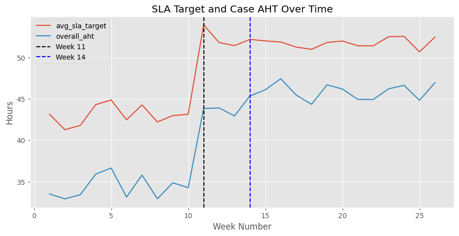
Review how the average SLA target trended against the AHT over time
Code
# Review the total resolution time and the respective SLA Target over timeops_cases_df.groupby(["week_number"]).agg( avg_sla_target=("sla_target_hours", "mean"), overall_aht=("resolution_hours", "mean"),).plot( title="SLA Target and Case AHT Over Time", xlabel="Week Number", ylabel="Hours", figsize=(11, 5),)plt.axvline(x=11, color="black", linestyle="--", label="Week 11")plt.axvline(x=14, color="blue", linestyle="--", label="Week 14")plt.legend()plt.show()
2. SLA Target and Case AHT Split
Split by Queue Name
Code
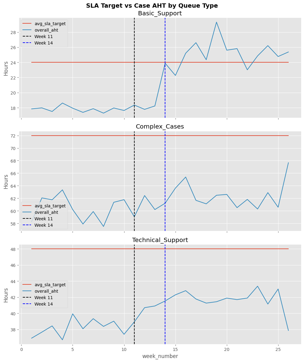
# Plot the SLA target and the total case handle time split by case typesfig, axes = plt.subplots(3, 1, figsize=(10, 12), sharex=True)fig.suptitle("SLA Target vs Case AHT by Queue Type", fontsize=14, fontweight="bold")for ax, queue inzip(axes, ["Basic_Support", "Complex_Cases", "Technical_Support"]): subset = ( ops_cases_df[ops_cases_df["queue_name"] == queue] .groupby("week_number") .agg( avg_sla_target=("sla_target_hours", "mean"), overall_aht=("resolution_hours", "mean"), ) ) subset.plot(ax=ax, title=queue, ylabel="Hours") ax.axvline(x=11, color="black", linestyle="--", label="Week 11") ax.axvline(x=14, color="blue", linestyle="--", label="Week 14") ax.legend()plt.tight_layout()plt.show()
Code
# Average Sla target by period and qeuue nameops_cases_df.groupby(["period", "queue_name"]).agg( avg_sla_target=("sla_target_hours", "mean"), overall_aht=("resolution_hours", "mean"),).round(2)
avg_sla_target
overall_aht
period
queue_name
Baseline
Basic_Support
24.0
17.77
Complex_Cases
72.0
60.24
Technical_Support
48.0
38.00
Self-serve Only
Basic_Support
24.0
18.21
Complex_Cases
72.0
59.53
Technical_Support
48.0
40.33
Both Changes
Basic_Support
24.0
25.15
Complex_Cases
72.0
62.69
Technical_Support
48.0
41.86
Split by Initial Handler Type
Code
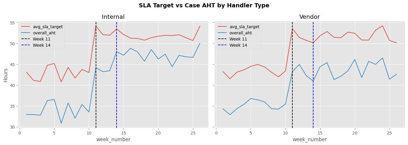
# Plot the SLA target and the total case handle time split by Initial Handler Typefig, axes = plt.subplots(1, 2, figsize=(14, 5), sharey=True)fig.suptitle("SLA Target vs Case AHT by Handler Type", fontsize=14, fontweight="bold")for ax, handler inzip(axes, ["Internal", "Vendor"]): subset = ( ops_cases_df[ops_cases_df["initial_handler_type"] == handler] .groupby("week_number") .agg( avg_sla_target=("sla_target_hours", "mean"), overall_aht=("resolution_hours", "mean"), ) ) subset.plot(ax=ax, title=handler, ylabel="Hours") ax.axvline(x=11, color="black", linestyle="--", label="Week 11") ax.axvline(x=14, color="blue", linestyle="--", label="Week 14") ax.legend()plt.tight_layout()plt.show()
Code
# Average Sla target by period and handler typeops_cases_df.groupby(["period", "initial_handler_type"]).agg( avg_sla_target=("sla_target_hours", "mean"), overall_aht=("resolution_hours", "mean"),).round(2)
avg_sla_target
overall_aht
period
initial_handler_type
Baseline
Internal
42.64
33.61
Vendor
43.25
34.77
Self-serve Only
Internal
52.32
43.08
Vendor
51.17
42.48
Both Changes
Internal
51.84
47.37
Vendor
51.83
43.93
Combined - Basic and Internal (most impact)
Code
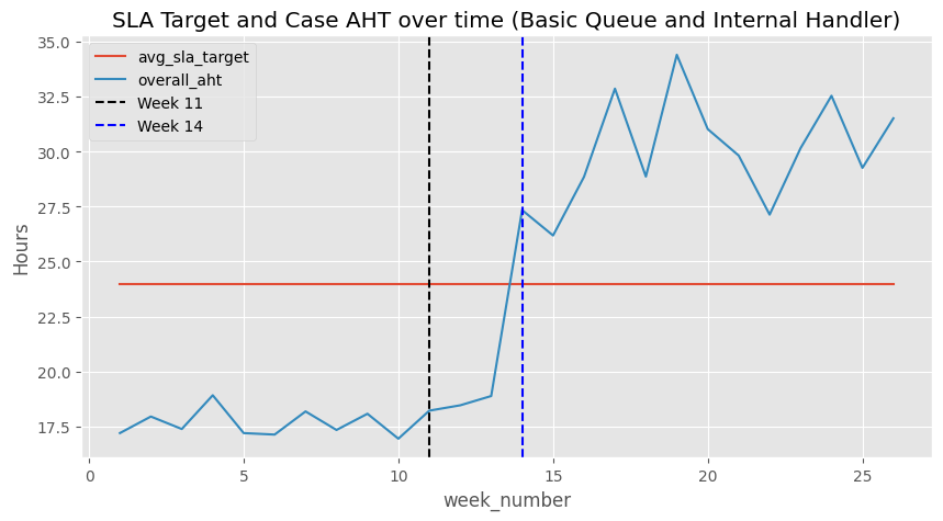
# Deep Dive into basic and internal AHT (both affected by changes)ops_cases_df[ (ops_cases_df["queue_name"] =="Basic_Support")& (ops_cases_df["initial_handler_type"] =="Internal")].groupby(["week_number"]).agg( avg_sla_target=("sla_target_hours", "mean"), overall_aht=("resolution_hours", "mean"),).plot( title="SLA Target and Case AHT over time (Basic Queue and Internal Handler)", ylabel="Hours", figsize=(10, 5),)plt.axvline(x=11, color="black", linestyle="--", label="Week 11")plt.axvline(x=14, color="blue", linestyle="--", label="Week 14")plt.legend()plt.show()
Check the distribution plots for the same.
Code
# Check the distribution of the cases to see if most cases are shifting or just a few skewing the averagefig, ax = plt.subplots(figsize=(12, 5))colors = {"Baseline": "steelblue","Self-serve Only": "orange","Both Changes": "crimson",}for period, color in colors.items(): subset = ops_cases_df[ (ops_cases_df["queue_name"] =="Basic_Support")& (ops_cases_df["initial_handler_type"] =="Internal")& (ops_cases_df["period"] == period) ]["resolution_hours"].dropna() kde = gaussian_kde(subset, bw_method=0.3) x = np.linspace(0, 100, 500) ax.plot(x, kde(x), label=period, color=color, linewidth=2) ax.fill_between(x, kde(x), alpha=0.15, color=color)ax.axvline(x=24, color="black", linestyle="--", linewidth=1.5, label="SLA Target (24h)")ax.set_title("Case Distribution — Basic Support, Internal Cases (Over Change Periods)", fontweight="bold",)ax.set_xlabel("Resolution Hours")ax.set_ylabel("Density")ax.legend()ax.set_xlim(0, 100)plt.tight_layout()plt.show()
3. ASA Analysis
Full Journey ASA
Code
# Review the full journey ASA at review levelops_reviews_df.groupby(["week_number_new"]).agg( asa_full_journey=("asa_hours", "mean"),).plot(title="Full Journey ASA over time", ylabel="Hours", figsize=(10, 4))plt.axvline(x=11, color="black", linestyle="--", label="Week 11")plt.axvline(x=14, color="blue", linestyle="--", label="Week 14")plt.legend()plt.show()
Code
# Review the full journey ASA at review level - basic and internal only ops_reviews_df[(ops_reviews_df['queue_name'] =='Basic_Support') & (ops_reviews_df['handler_type'] =='Internal')].groupby(["week_number_new"]).agg( asa_full_journey=("asa_hours", "mean"),).plot(title="Full Journey ASA over time (Basic Internal only)", ylabel="Hours", figsize=(10, 4))plt.axvline(x=11, color="black", linestyle="--", label="Week 11")plt.axvline(x=14, color="blue", linestyle="--", label="Week 14")plt.legend()plt.show()
Code
# Plot the first touch ASA and the total case handle time split by case typesfig, axes = plt.subplots(3, 1, figsize=(7, 11), sharex=True)fig.suptitle("Full Journey ASA by Queue Type", fontsize=14, fontweight="bold")for ax, queue inzip(axes, ["Basic_Support", "Complex_Cases", "Technical_Support"]): subset = ( ops_reviews_df[ops_reviews_df["queue_name"] == queue] .groupby("week_number_new") .agg( full_asa=("asa_hours", "mean"), ) ) subset.plot(ax=ax, title=queue, ylabel="Hours") ax.axvline(x=11, color="black", linestyle="--", label="Week 11") ax.axvline(x=14, color="blue", linestyle="--", label="Week 14") ax.legend()plt.tight_layout()plt.show()
Code
# Plot the full journey ASA and the total case handle time split by Handler Typefig, axes = plt.subplots(1, 2, figsize=(14, 5), sharey=True)fig.suptitle("Full Journey ASA by Handler Type", fontsize=14, fontweight="bold")for ax, handler inzip(axes, ["Internal", "Vendor"]): subset = ( ops_reviews_df[(ops_reviews_df["handler_type"] == handler)] .groupby("week_number_new") .agg(full_asa=("asa_hours", "mean")) ) subset.plot(ax=ax, title=handler, ylabel="Hours") ax.axvline(x=11, color="black", linestyle="--", label="Week 11") ax.axvline(x=14, color="blue", linestyle="--", label="Week 14") ax.legend()plt.tight_layout()plt.show()
First Touch ASA
Code
# Review the first touch ASA at review levelops_reviews_df[ops_reviews_df["review_order"] ==1].groupby(["week_number_new"]).agg( asa_full_journey=("asa_hours", "mean"),).plot(title="First Touch ASA over time", ylabel="Hours", figsize=(10, 4))plt.axvline(x=11, color="black", linestyle="--", label="Week 11")plt.axvline(x=14, color="blue", linestyle="--", label="Week 14")plt.legend()plt.show()
Code
# Plot the First Touch ASA and the total case handle time split by case typesfig, axes = plt.subplots(3, 1, figsize=(7, 11), sharex=True)fig.suptitle("First Touch ASA by Queue Type", fontsize=14, fontweight="bold")for ax, queue inzip(axes, ["Basic_Support", "Complex_Cases", "Technical_Support"]): subset = ( ops_reviews_df[ (ops_reviews_df["queue_name"] == queue)& (ops_reviews_df["review_order"] ==1) ] .groupby("week_number") .agg( full_asa=("asa_hours", "mean"), ) ) subset.plot(ax=ax, title=queue, ylabel="Hours") ax.axvline(x=11, color="black", linestyle="--", label="Week 11") ax.axvline(x=14, color="blue", linestyle="--", label="Week 14") ax.legend()plt.tight_layout()plt.show()
Code
# Plot the first touch ASA and the total case handle time split by Handler Typefig, axes = plt.subplots(1, 2, figsize=(14, 5), sharey=True)fig.suptitle("First Touch ASA by Handler Type", fontsize=14, fontweight="bold")for ax, handler inzip(axes, ["Internal", "Vendor"]): subset = ( ops_reviews_df[ (ops_reviews_df["handler_type"] == handler)& (ops_reviews_df["review_order"] ==1) ] .groupby("week_number_new") .agg(full_asa=("asa_hours", "mean")) ) subset.plot(ax=ax, title=handler, ylabel="Hours") ax.axvline(x=11, color="black", linestyle="--", label="Week 11") ax.axvline(x=14, color="blue", linestyle="--", label="Week 14") ax.legend()plt.tight_layout()plt.show()
# Plot the review and the total case handle time split by case typesfig, axes = plt.subplots(3, 1, figsize=(10, 12), sharex=True)fig.suptitle("Review Level AHT by Queue Type", fontsize=14, fontweight="bold")for ax, queue inzip(axes, ["Basic_Support", "Complex_Cases", "Technical_Support"]): subset = ( ops_reviews_df[ops_reviews_df["queue_name"] == queue] .groupby("week_number_new") .agg( review_aht=("aht_minutes", "mean"), ) ) subset.plot(ax=ax, title=queue, ylabel="Minutes") ax.axvline(x=11, color="black", linestyle="--", label="Week 11") ax.axvline(x=14, color="blue", linestyle="--", label="Week 14") ax.legend()plt.tight_layout()plt.show()
Code
# Plot the first touch ASA and the total case handle time split by Handler Typefig, axes = plt.subplots(1, 2, figsize=(14, 5), sharey=True)fig.suptitle("Review Level AHT by Handler Type", fontsize=14, fontweight="bold")for ax, handler inzip(axes, ["Internal", "Vendor"]): subset = ( ops_reviews_df[ops_reviews_df["handler_type"] == handler] .groupby("week_number_new") .agg(full_asa=("aht_minutes", "mean")) ) subset.plot(ax=ax, title=handler, ylabel="Minutes") ax.axvline(x=11, color="black", linestyle="--", label="Week 11") ax.axvline(x=14, color="blue", linestyle="--", label="Week 14") ax.legend()plt.tight_layout()plt.show()
Section Summary
Four metrics were used to diagnose where time is being lost across the case lifecycle: case-level AHT (total resolution hours), review-level AHT (active agent handle time per touch), first-touch ASA (wait before initial assignment), and full journey ASA (cumulative wait across all touches). All of these together can differentiate between separate queue delay, active handling, and rework as distinct contributors to SLA deterioration.
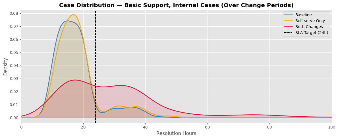
Case-level AHT shows the overall time increase for work: Basic_Support resolution hours rose from ~18 hours at baseline to ~25–30 hours post Week 14 — the only queue where AHT continously breached its 24-hour SLA target. Complex and Technical queues also rose in absolute terms but remained within their respective targets. The KDE distribution confirms this is a systemic shift across all Basic cases, not an outlier effect.
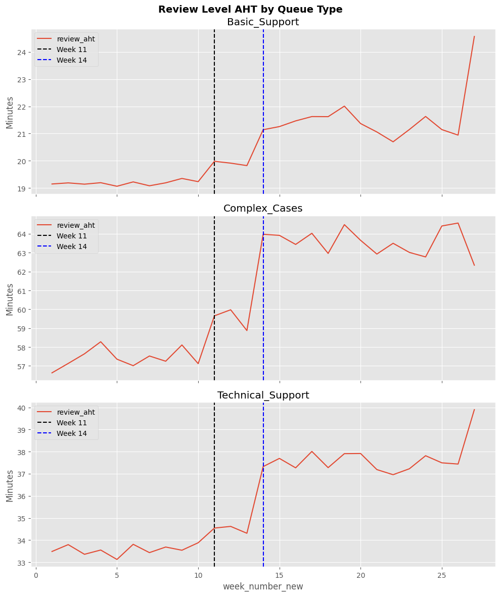
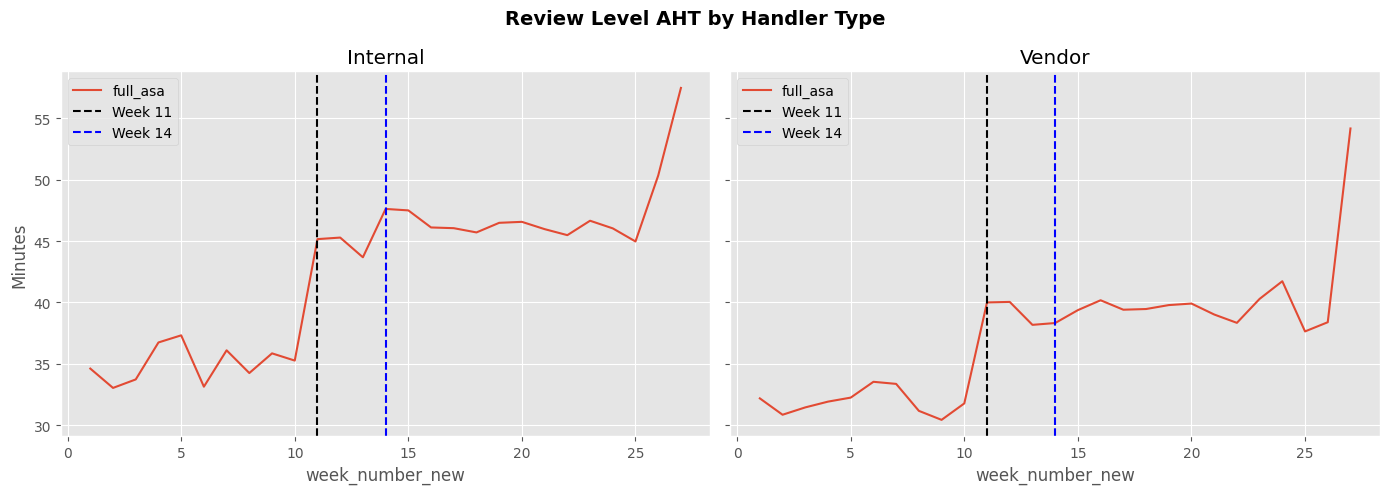
Review-level AHT reveals the complexity mix effect: Per-review active handle time increased for all three queues and both handler types after Week 11 — Basic_Support from ~19 to ~21 minutes, Complex_Cases from ~57 to ~64 minutes, Technical_Support from ~33 to ~38 minutes. Additionally, both internal and vendor groups moved together at Week 11, ruling out routing as the cause. Agents are spending more time per touch because the remaining cases are genuinely harder which is a direct consequence of self-serve deflecting the simpler work.
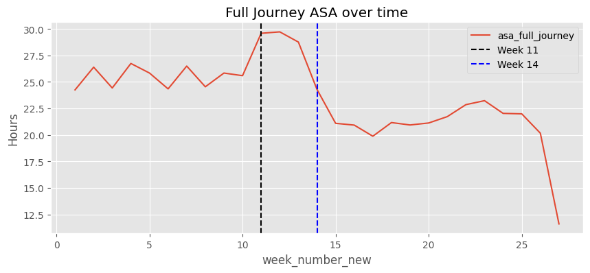
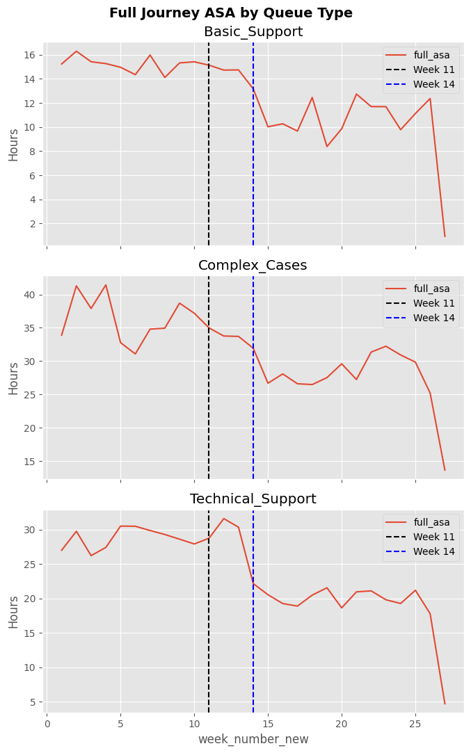
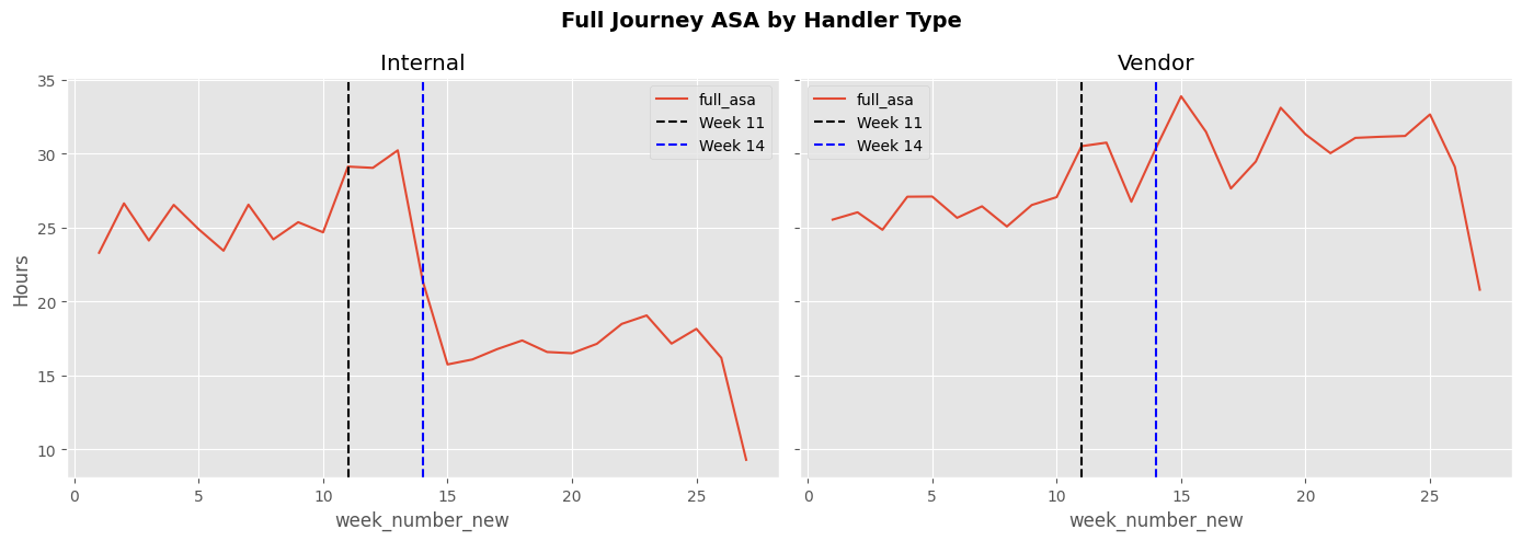
ASA analysis produced a counterintuitive finding: First-touch and full-journey ASA both spiked at Week 11 then declined after Week 14 — meaning cases were being assigned faster after routing was introduced, not slower. This rules out understaffing or slow assignment as the bottleneck and reframes the problem entirely: routing improved assignment speed while simultaneously degrading assignment quality. This requires additional review of other metrics now.
The gap between case-level and review-level AHT is a rework signal: Each individual review didn’t become dramatically slower after routing. We need to analyze what went wrong in terms of individual reviews causing overall delay in case resolution time. One potential direction is - additional touches, each preceded by another queue wait, could accumulate into resolution times that breach the SLA target. The issue might be is rework, not slowness.
Next: The next step is to analyze case-level and review-level outcomes. I will look at average number of reviews, sent back rates, escalation rates, first time resolution rates etc.