This section examines how SLA performance evolved across the three periods, segmented by handler type and queue. The goal is to establish whether the decline is explained by the complexity mix shift alone, or the routing or whether it was some combination of both.
There is a detailed summary section at the end.
Imports and Setup
This is similar across all files
Code
import pandas as pdimport matplotlib.pyplot as pltimport warningswarnings.filterwarnings("ignore")# Set plt styleplt.style.use("ggplot")# Load the operations cases and reviews dataops_cases_df = pd.read_csv("ops_cases.csv")ops_reviews_df = pd.read_csv("ops_reviews.csv")# Set the period order for the dataperiod_order = ["Baseline", "Self-serve Only", "Both Changes"]ops_cases_df["period"] = pd.Categorical( ops_cases_df["period"], categories=period_order, ordered=True)
1. Overall SLA Trend
Weekly SLA Trend in the data
Code
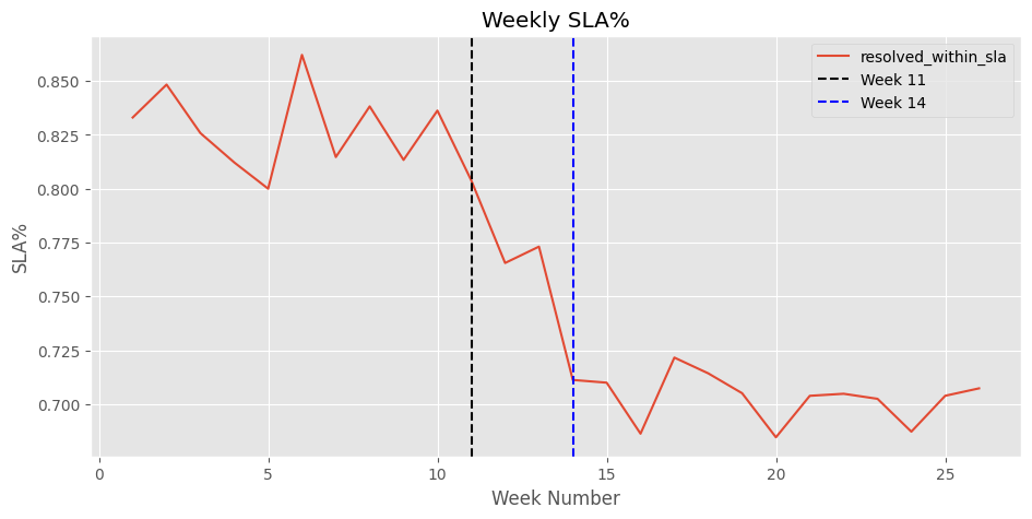
# Plot the weekly graph and specifically mark Week 11 and Week 14weekly_sla_df = ( ops_cases_df[["resolved_within_sla", "week_number"]].groupby("week_number").mean()).plot(xlabel="Week Number", ylabel="SLA%", title="Weekly SLA%", figsize=(11, 5))plt.axvline(x=11, color="black", linestyle="--", label="Week 11")plt.axvline(x=14, color="blue", linestyle="--", label="Week 14")plt.legend()plt.show()
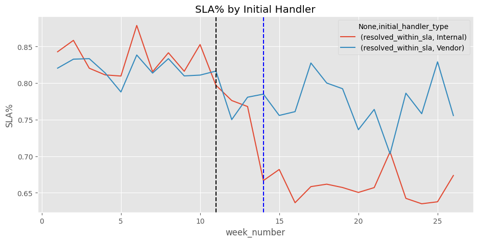
Internal and vendor SLA are compared across all three periods.
Code
# Review if there were any volume trends by handler typequeue_name_sla_df = ( ops_cases_df[["resolved_within_sla", "initial_handler_type", "week_number"]] .groupby(["initial_handler_type", "week_number"], as_index=False) .mean())queue_name_sla_df.pivot(index="week_number", columns="initial_handler_type").plot( figsize=(11, 5), ylabel="SLA%", title="SLA% by Initial Handler")plt.axvline(x=11, color="black", linestyle="--", label="Week 11")plt.axvline(x=14, color="blue", linestyle="--", label="Week 14")
SLA by Vendor Type
Code
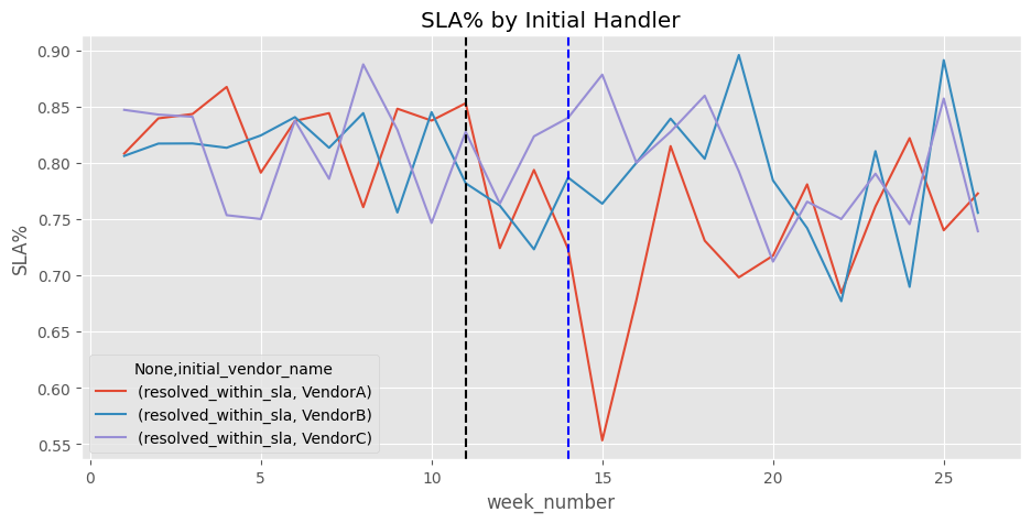
# Was there any difference between the three vendorsqueue_name_sla_df = ( ops_cases_df[~ops_cases_df["initial_vendor_name"].isna()][ ["resolved_within_sla", "initial_vendor_name", "week_number"] ] .groupby(["initial_vendor_name", "week_number"], as_index=False) .mean())queue_name_sla_df.pivot(index="week_number", columns="initial_vendor_name").plot( figsize=(11, 5), ylabel="SLA%", title="SLA% by Initial Handler")plt.axvline(x=11, color="black", linestyle="--", label="Week 11")plt.axvline(x=14, color="blue", linestyle="--", label="Week 14")
3. SLA by Queue Type
Code
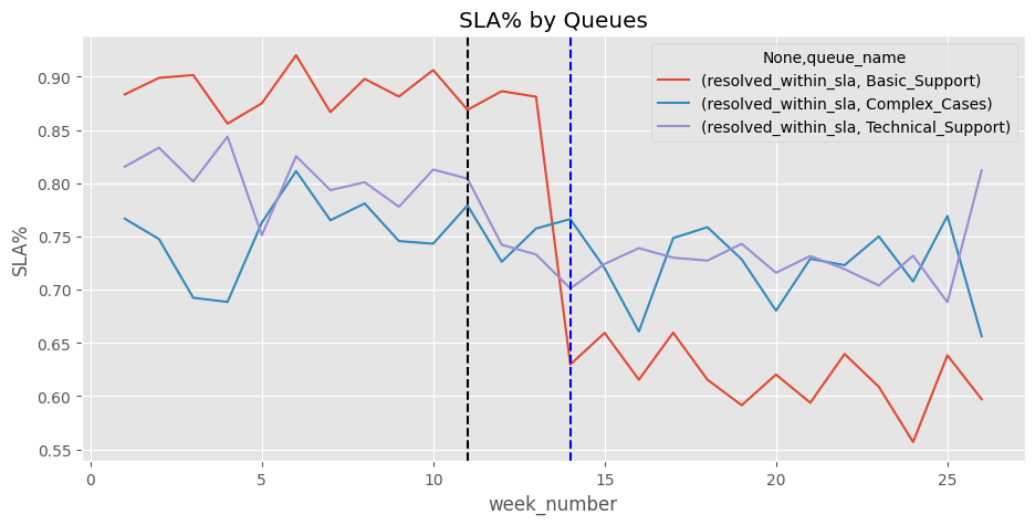
# Review if there were any volume trends by categorical variables like queue_name and initial_handler_type as well as the periodqueue_name_sla_df = ( ops_cases_df[["resolved_within_sla", "queue_name", "week_number"]] .groupby(["queue_name", "week_number"], as_index=False) .mean())queue_name_sla_df.pivot(index="week_number", columns="queue_name").plot( figsize=(11, 5), ylabel="SLA%", title="SLA% by Queues")plt.axvline(x=11, color="black", linestyle="--", label="Week 11")plt.axvline(x=14, color="blue", linestyle="--", label="Week 14")
Section Summary
Overall SLA declined from ~83% in the baseline period to ~70% after both changes were live, a 13-pp drop. The decline happened in two visible steps, first at Week 11 and then more sharply after Week 14, suggesting both changes contributed rather than one isolated event.
The self-serve automation triggered the first dip: Between Weeks 11 and 13, SLA fell from ~83% to ~79%. This is consistent with the complexity mix shift identified in the volume section: Since Basic_Support cases were deflected, agents inherited a harder caseload, putting natural upward pressure on resolution times even before the routing change. We can further verify it from the resolution time graphs in the next section.
The routing change drove the sharper, sustained decline: Post Week 14, SLA dropped further to ~70% and stabilised there. This second dip is not explained by volume or mix alone since those were already stable by this point.
Splitting by handler type reveals important findings: Internal and vendor SLA tracked almost identically during the baseline period (both around 82-84%). After Week 11 both dipped modestly and in parallel. But after Week 14 they diverge sharply — internal SLA falls to 66% while vendor holds at 77%. Since routing only affected internal teams, this divergence could be a strong evidence that routing is the primary driver of the post-Week 14 decline.
Queue-level SLA tells the same story: Basic_Support SLA, which was the highest pre-change at ~89%, collapses most severely post Week 14 to 62%. What could have potentially happened is that basic cases that previously got resolved quickly by any available agent are now waiting in specialist queues they don’t need to be in. This will be further reviewed through the AHT and ASA analysis.
Vendor performance was not uniform: This is another interesting finding - VendorA is showing a notable dip around Week 14 before recovering. This could be a limitation when using vendor teams as a control group in the causal analysis. Not focussing on this as of now but something to keep in mind.
Next: The next step is the AHT and ASA analysis to see how the impact of the changes affected the time taken to start working on a case and to resolve a cse.